Operational Side Conditions
Operational Side Conditions are a group of components that influence the operating performance of controllable systems. These components either specify limitations in the mode of operation, or a certain operational behavior is allocated costs or profits in order to put it at a disadvantage or to give preference to it in optimization. The individual components are described under Operational Side Conditions. All these components are to be found as templates in the Component template library folder Operational Side Conditions.
This article deals with Operational Side Conditions using the example of an application case.
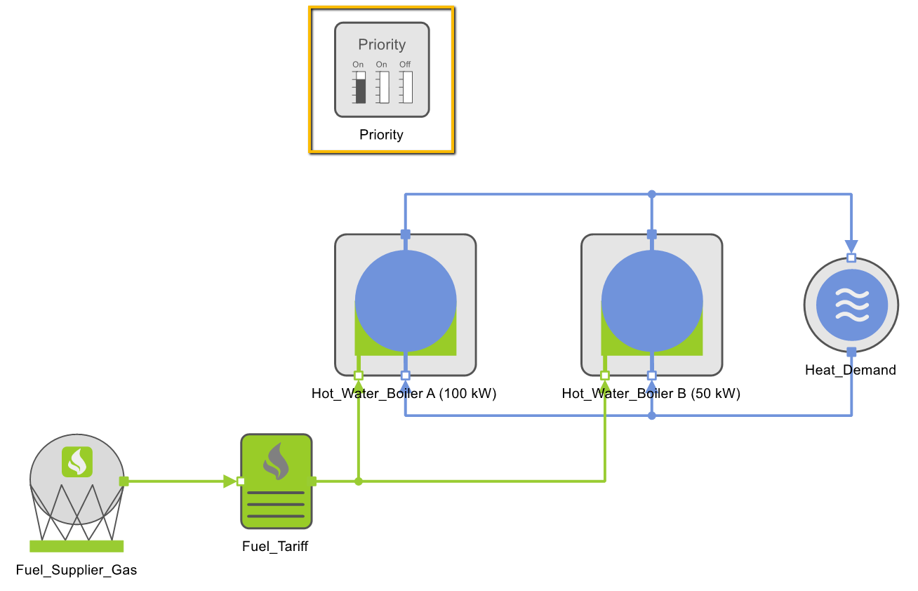
Example Energy System and Components Used
The example energy system illustrated in the following figure consists of two boilers with a nominal output of 100 and 50 kW each, which cover a specified heat requirement. The behavior of this system shall be influenced according to the wishes of the user. For this purpose, six operational side conditions are defined by the associated components. The selection of side conditions and their effects on the process are explained individually below.
Priority (switch-on sequence)
The controllable systems should be switched on according to a specified order, since one generator, for example, is to cover the base load and another the peak load. This rule can be mapped with the component Priority from the Component template library folder Operational Side Conditions.
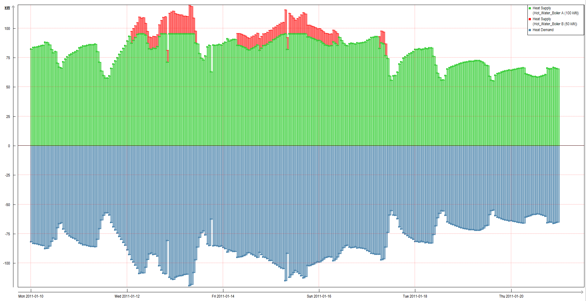
In this example, the order in which the boilers are switched on is determined to produce the required heat. Hot water boiler A (100 kW) is given Priority 1: As long as the heat demand does not exceed the nominal output of boiler A, only this boiler is used for heat production. Hot water boiler B (50 kW) should only be switched on if heat demand exceeds 100 kW.
This course can also be seen in the time series shown below. The blue area represents the total heat demand, and the green and red one, the heat generation of the hot water boiler A and B, respectively. Due to the Minimum Part Load of 20 % or 10 kW set for boiler B, boiler B may be switched on even if boiler A has not yet reached its rated output of 100 kW. Boiler B should not produce a heat output lower than 10 kW, so that boiler B’s share of the heat demand of more than 100 kW must be at least 10 kW.
Availability
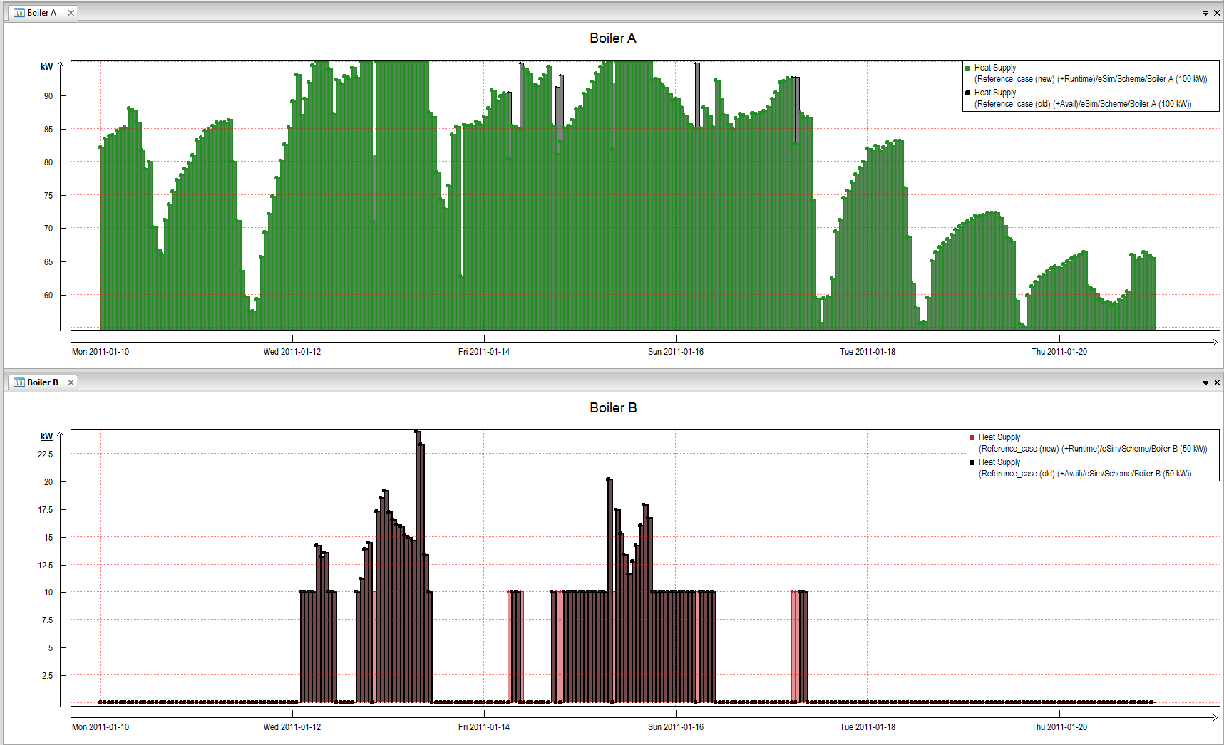
Next, the user wants to map a limited availability of an unit in the model. This may be necessary in practice, for example due to an audit.
The component Availability from the Component template library folder Operational Side Conditions is used for this purpose. The Adjustable Component is selected in the Availability component. The availability limit (absolute or relative to the maximum power) is then assigned to it. In this example, the maximum output of boiler A is reduced to 95 kW. The resulting new courses of the heat output of both boilers are displayed in color in comparison to the previous black-marked gradients: Hot water boiler A – green, hot water boiler B – red.
In most cases, boiler A produces only 5 kW less heat in the peaks than in the previous example. This difference is compensated by boiler B in a similiar way as in the previous example. Sometimes, however, this slight reduction in availability can also lead to a more frequent switch-on or prolonged operation of boiler B, as can be seen in the figure below.

Operating Time Parameters: Minimum Runtime and Downtime
Up to now, the switching on behavior of the two hot water boilers was only influenced by the set priority and the respective existing heat demand. As soon as demand dropped to base-load level, peak-load boiler B could be switched off. This “opportunistic” behavior does not always make sense in reality, as it can be uneconomical to let a system run for such a short period of time. On the other hand, it may also not be advisable or technically possible to switch on a system that has just been switched off.
This correlation can be mapped in the component Operating Time Parameters from the Component template library folder Operational Side Conditions. In the example energy system, hot water boiler B was “forbidden” to be in operation or at a standstill for less than 4 hours. The effects compared to the previous process are shown below: Individual 2-hour operations were extended to 4 hours, downtime gaps were filled. In both cases, the base load boiler A had to deliver less.
For this component, it is necessary to set a look-ahead of at least the duration of the set minimum operating time or standstill time.
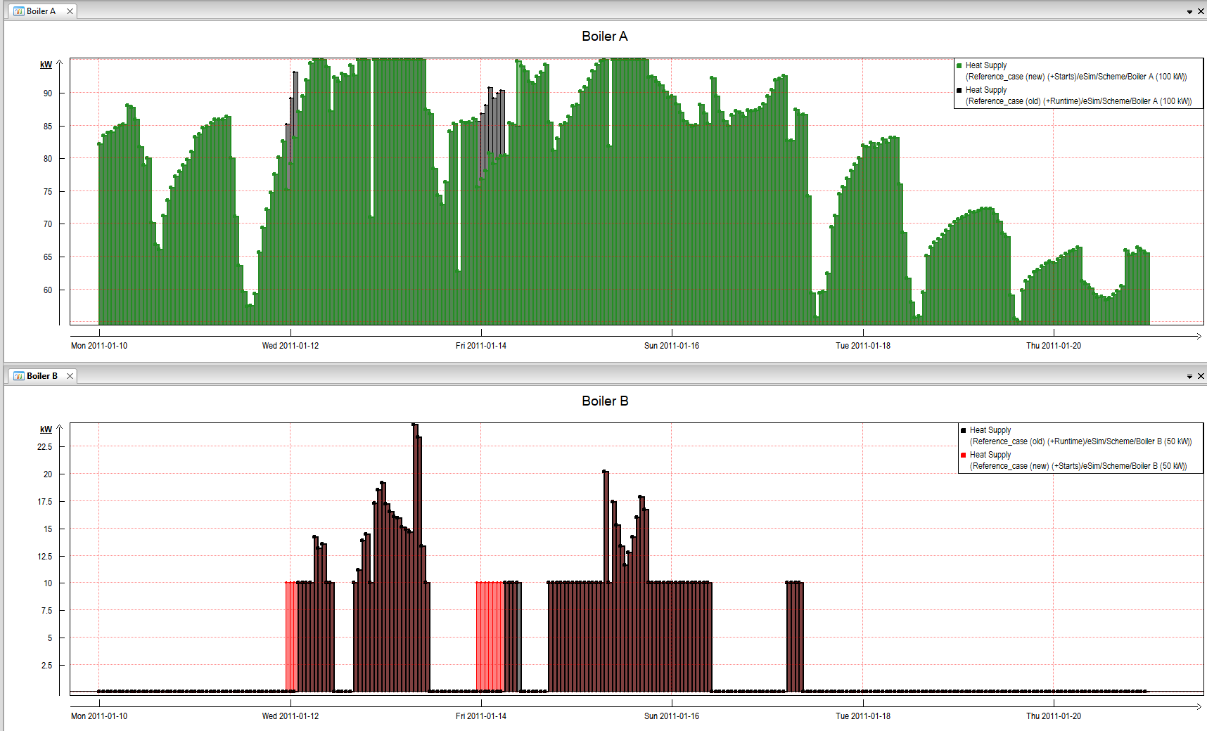
Number of Starts per Day
The Operating Time Parameters described in the previous section have an indirect effect on the number of starts: if it is foreseeable that a system would have to be restarted before the end of its minimum downtime, it will not be shut down. However, you can also restrict the maximum number of daily starts directly by setting it in the component Number of Starts from the Component template library folder Operational Side Conditions.
In this example, the setting for hot water boiler B has been set to 1. The illustration below shows that for hot water boiler B, which is only allowed to start once a day, in the first case the start is brought forward to 23:00 on the previous day, in order to be allowed to start again on the following day. In the second case, boiler B is not stopped because its maximum number of daily starts has already been reached.
For the component Number of Starts, it is necessary to set a look-ahead of at least 24 h.
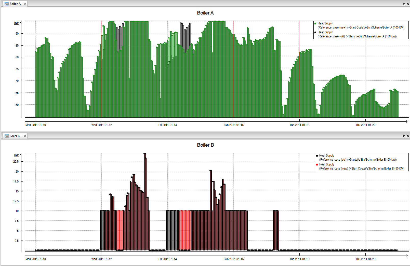
Start Costs
Another approach for the indirect control of startup processes is their allocation with costs. In reality, this can mean, for example, additional fuel costs for starting processes.
Use the Start Costs component from the Component template library folder Operational Side Conditions. In the Start Costs form, select the Controllable Component and enter the monetary value per start operation in EUR next to Start Costs Component. Then the selected system only starts if the expected added value exceeds the entered start costs (and no side conditions are violated otherwise).
In the present example, this results in a stop waiver, because a further start would entail more costs than benefits. The number of starts for boiler B is reduced from 9 to 3 in comparison with the status after using the Availability component.
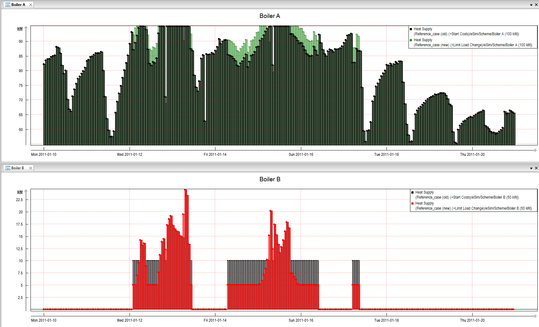
Limit Load Change
The last here presented possibility of influencing the operation of a controllable system is the specification of a limit load change. The Limit Load Change component is also located as a template in the Component template library folder Operational Side Conditions. This component contains Maximum Power Change Positive and Maximum Power Change Negative per time unit, i.e., the maximum permissible increase or decrease in power per time step. Possible units are kW/h, kW/15 min or MW/day.
For example, a power generator may not start or end feeding into the grid arbitrarily fast or abruptly, because there may be instabilities in the grid.
In the following example, boiler B was set to increase heat generation by no more than 5 kW per hour. For this purpose, the previously discussed Minimum Part Load had to be reduced from 10 to 5 kW, as otherwise the step from 0 to 5 kW would not be possible.
The figure shows a smoother generation course for both boilers when hot water boiler B is in operation.
For the component Limit Load Change, it is necessary to set a look-ahead of at least the duration of the set load change.