Parameter Study
In this article you will learn how to investigate the change in economic parameters (here: amortization time and net present value) depending on the electricity price. The example is based on the Tutorial 70: Variable Price of Electricity.
The Example Energy System
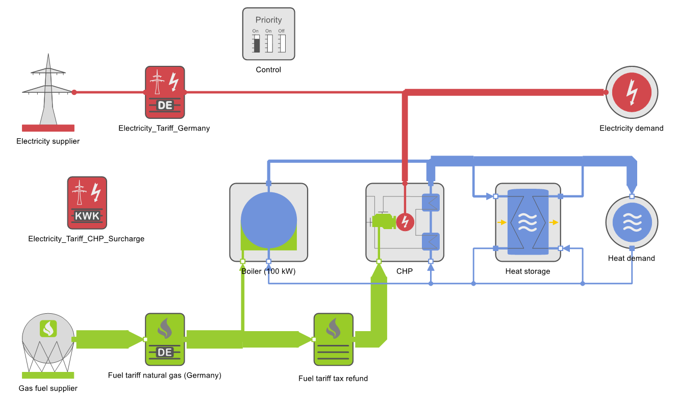
In the example, a simple energy system with two boilers (100 kW and 50 kW) serves as the Reference case. In a first version, the smaller boiler is replaced by a cogeneration plant (CHP) with the corresponding Nominal thermal capacity. In a second version, this system is supplemented by a 500 kWh storage (see following figure). Using Variant comparison, the Reference case is compared economically to the two variants.
Creating a Sensitivity Analysis
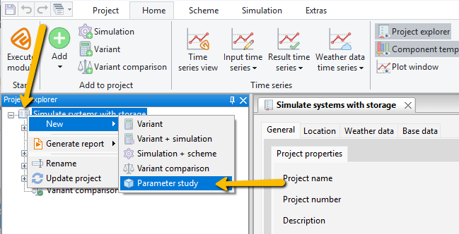
To add a sensitivity analysis to the project, an Parameter study node is created in the Project explorer as follows:
Right-click on the project node ![]() in the Project explorer, select New →
in the Project explorer, select New → ![]() Parameter study.
Parameter study.
Configuring the Variable Parameter
If the newly created ![]() Parameter study node is selected in the project explorer, the Input requirements form opens in the form view (right) under the Settings tab.
Parameter study node is selected in the project explorer, the Input requirements form opens in the form view (right) under the Settings tab.
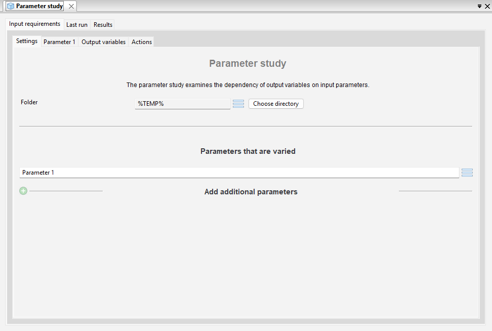
In it, first select the Folder where you want to save the results of the Parameter study as a CSV file.
To vary the electricity price (Working price and Grid usage charge), proceed as follows.
To select the parameter, a window opens, which displays the form of the selected component.
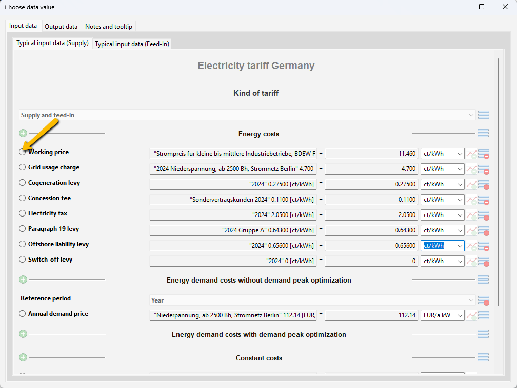
The window then closes.
This loads the current entries of the Working price into Lower limit and Upper limit fields.
![]() Add a further coupled parameter: Grid usage charge. In this example, the working prices and grid usage charges do not differ in the variants.
Add a further coupled parameter: Grid usage charge. In this example, the working prices and grid usage charges do not differ in the variants.
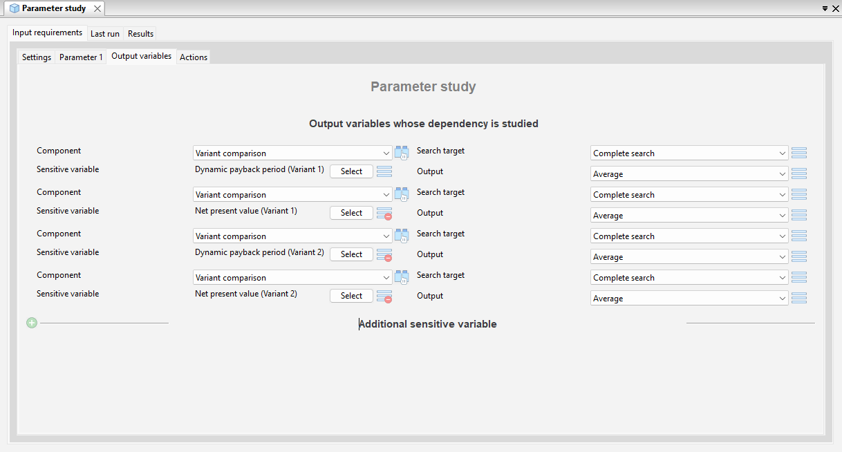
Selecting Sensitive Variables (output variables)
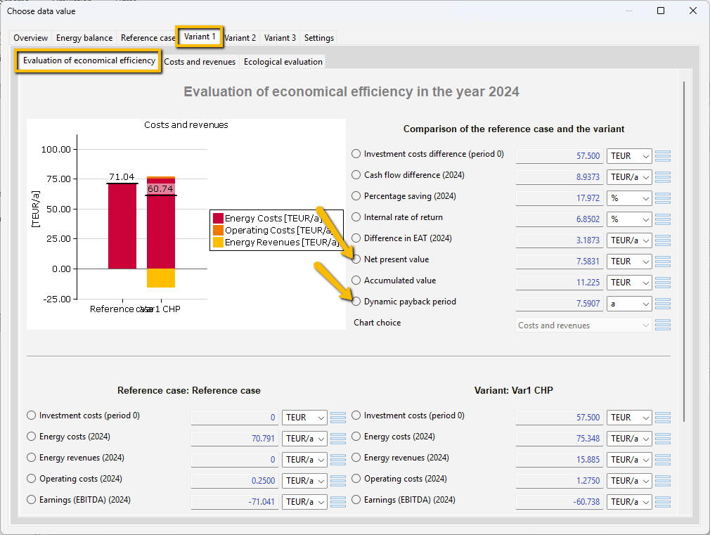
The next step is to select the Output variables whose dependency on the variable parameters is studied in the Parameter study. The selection is made under the tabs Input requirements → Ouput variables. Up to 10 values can be specified. In our example, the Dynamic payback period and the Net present value in the economic evaluation of variants 1 and 2 are selected.
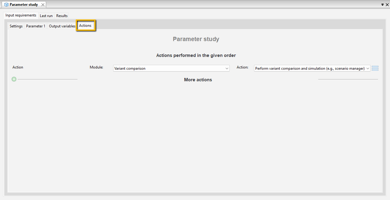
Actions to be Performed
Finally, under the tabs Input requirements → Actions, define which steps are to be carried out per iteration in the parameter study, in our example: Perform variant comparison and simulation (e.g., scenario manager).
Performing the Parameter Study
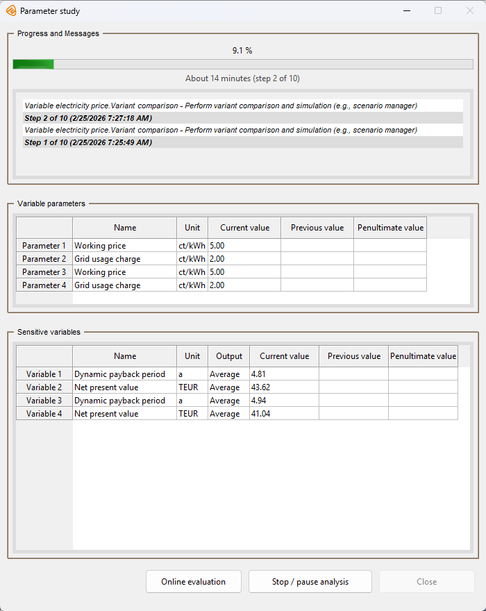
Now start the Parameter study by pressing the TOP-Energy button ![]() in the ribbon (Execute module). Alternatively, you can also use the shortcut <Ctrl>+<T>. All actions are performed in the given order for each sampled value of the variable parameter. During the run, a dialog box appears that informs you of the progress and displays current intermediate results. If necessary, the analysis can be paused or aborted at the bottom right.
in the ribbon (Execute module). Alternatively, you can also use the shortcut <Ctrl>+<T>. All actions are performed in the given order for each sampled value of the variable parameter. During the run, a dialog box appears that informs you of the progress and displays current intermediate results. If necessary, the analysis can be paused or aborted at the bottom right.
Visualizing Results
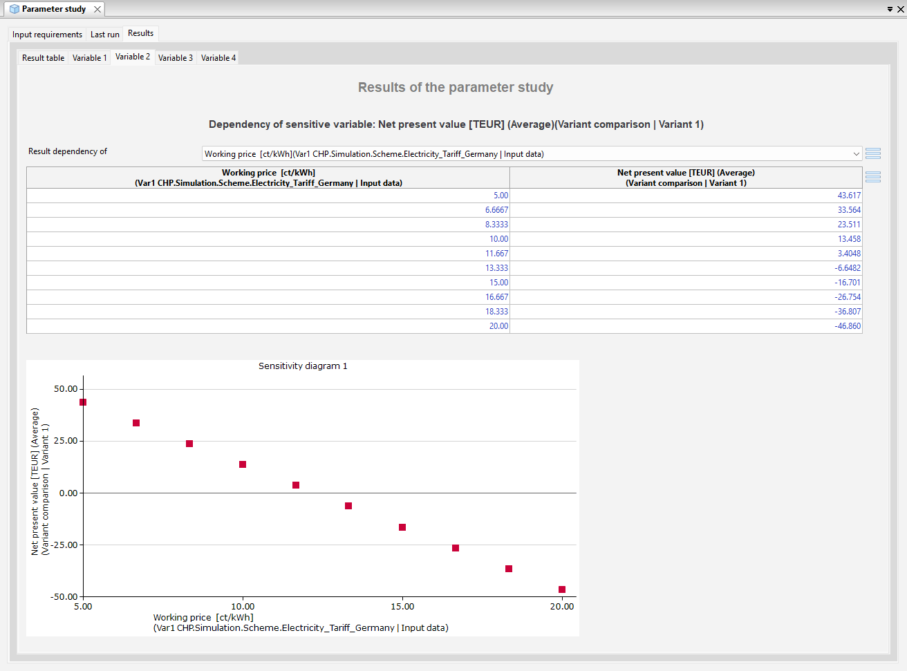
If the Parameter study has been carried out successfully, the Results can then be viewed under the tab of the same name. Here, for each sensitive variable, its dependence on the variable parameters is displayed in tabular and diagram form (see the following figure).
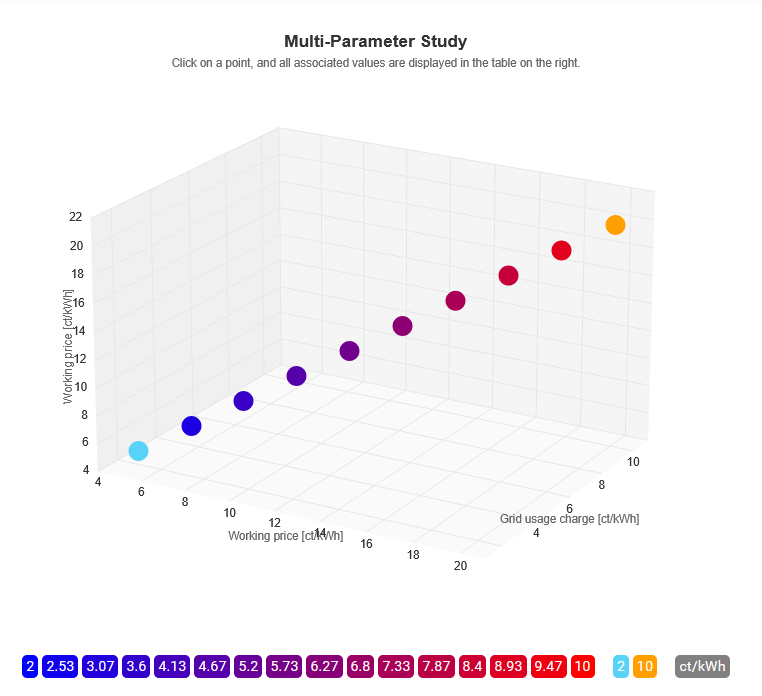
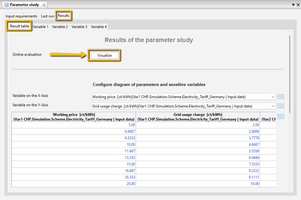
In addition, you can comfortably visualize the results saved in the CSV file with an online tool. You open this tool with the button Visualize under the tab Result table behind the identifier Online evaluation (see following figure).
The TOP-Energy tool for variation calculations opens in your browser (see the following figure).
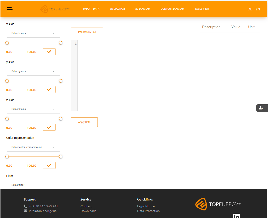
Insert the result data of the parameter study via right-click and the context menu directly from the clipboard. Alternatively, upload the saved CSV file. Make the desired settings for the axes, filters, and color display on the left side.