Mixing Temperature Specifications of Heat Generators Connected in Parallel at Different Temperature Levels
This article describes how in TOP-Energy an energy system with two or more heat generators connected in parallel with different flow temperatures is simulated in such a way that a certain mixture temperature is not undershot. Due to the Special Features of Heat, components of the Programmable Control are used for this purpose in TOP-Energy.
The article is aimed at experienced TOP-Energy users because the complex issues require a profound understanding of the simulation and optimization processes.
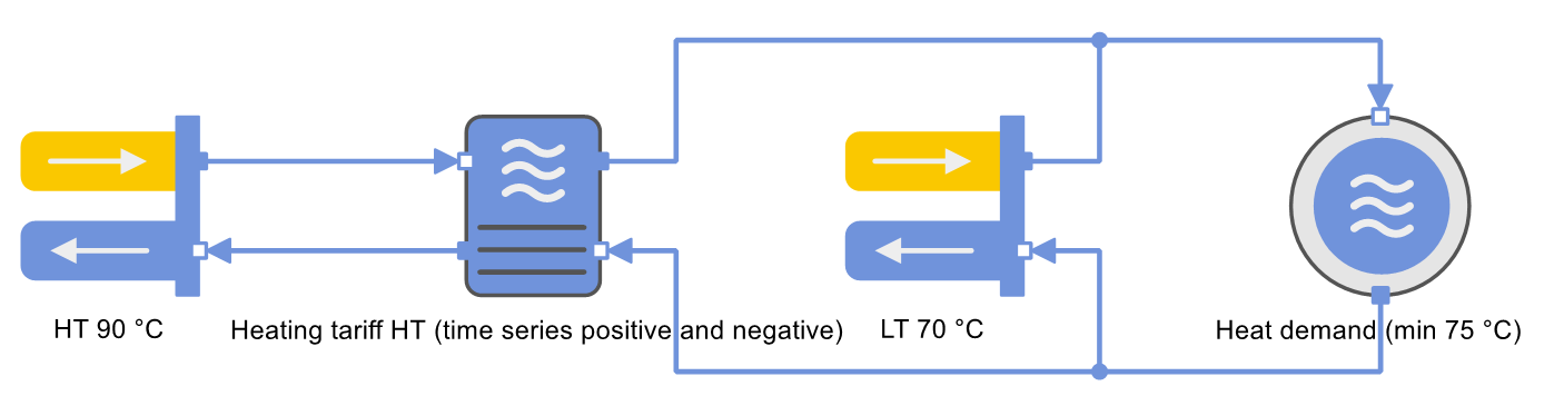
The energy system in the following figure illustrates the problem.
The minimum ratio of the heat quantities to be generated with high and low temperature is calculated using the previously known flow and set temperatures. This ratio is a linear bound in the optimization problem.
The application is not limited to heat. The principles can also be transferred to cooling networks.
A similar solution principle to the one presented here is shown in the Tutorial on Heat Generators at Different Temperature Levels for Series Connection. Although the basic principle of derivation is the same, a distinction must be made between parallel and series connection.
Description of the Problem Using an Example
A heat demand with a minimum inlet temperature of 75 °C shall be covered by two heat generators, a high temperature heat generator (HT) with a flow temperature of 90 °C, and a low temperature heat generator (LT) with a flow temperature of 70 °C. The low-temperature heat generator cannot cover the heat demand alone, because the minimum temperature of 75 °C is not reached. Because the low-temperature heat is free of charge and the high-temperature heat comes with a price, it is necessary to calculate the optimum (most cost-effective) mixture.
In energy system optimization, in order to avoid non-linear problems, the mixture temperature is not used as an optimization variable, but is indirectly determined by a lower bound for the ratio of low and high temperature heat quantities. In TOP-Energy the problem is solved with the help of the control components as follows:
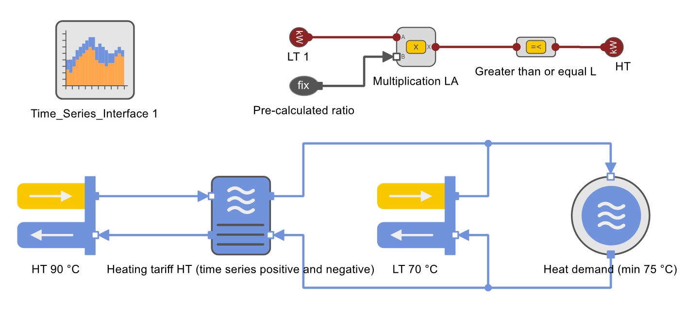
The graphical control elements represent the following equation:
\( \begin{equation} \begin{aligned} \dot{Q}_{HT} \ge c \cdot \dot{Q}_{LT} && \qquad(1)\\[.3cm] \end{aligned}\end{equation} \),
in which \( c \) is a constant which is entered in the form of the component named as the Ratio calculated in advance. The calculation rule follows below in the section Calculation of the Heat Ratio.
In the tutorial, the following time series is stored as input value for the price of high-temperature heat (in the heat tariff):
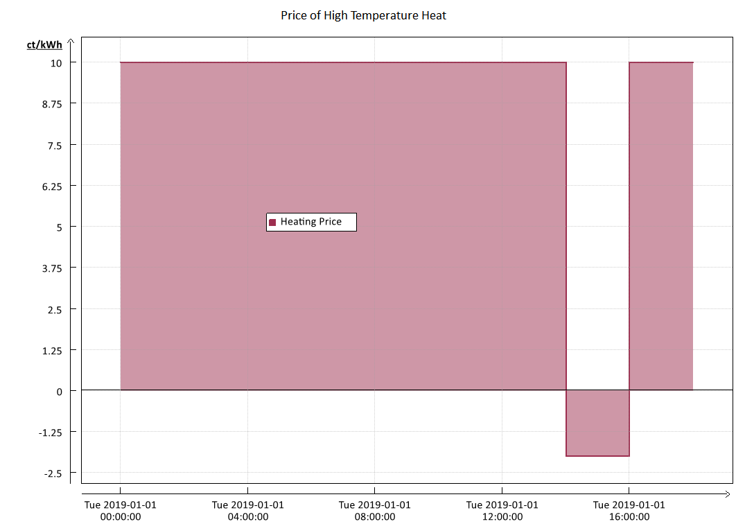
In the simulation period of several hours, the heat price is constantly 9 ct/kWh, only in the penultimate time step it has a negative value and is thus converted into revenue.
The following figure shows the optimized result of the simulation for the produced Heat and the Inlet Temperature at the Heat Demand.
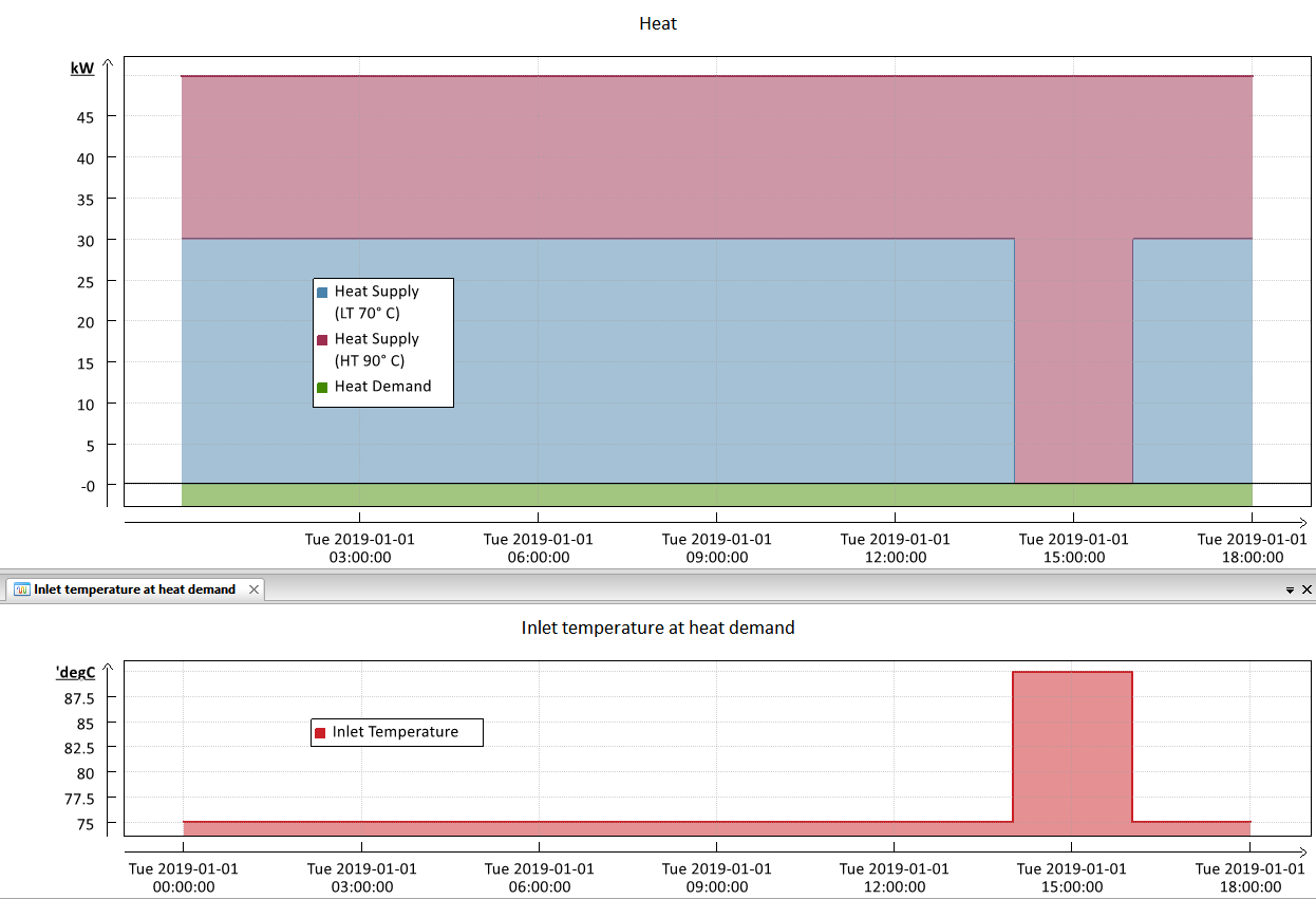
The specification that the Inlet Temperature at the Heat Demand must be at least 75 °C is observed.
In contrast to the normal case of a positive heat price, in which only so much expensive high-temperature heat is used that the specified minimum 75 °C is reached, only high-temperature heat is used in the time step of the negative heat price. This is because revenues are generated by the negative price and these are maximized within the scope of optimization. Therefore, at the time of the negative heat price, the inlet temperature at the heat demand is higher than 75 °C. This shows that TOP-Energy also optimizes the energy system within the given limits, here the minimum inlet temperature of 75 °C.
Calculation of the Heat Ratio
If the temperatures of the producers are not constant and therefore provided with a time series, \( c \) is also not a constant over the simulation period. In this case \( c \) changes with the temperature conditions. It is possible to calculate and specify a time series for \( c \) in advance, but the direct temperature-dependent calculation of the ratio \( c \) in TOP-Energy is much more flexible.
As an example, the following figure shows the same model with a high-temperature and a low-temperature heat generator with varying flow temperature.
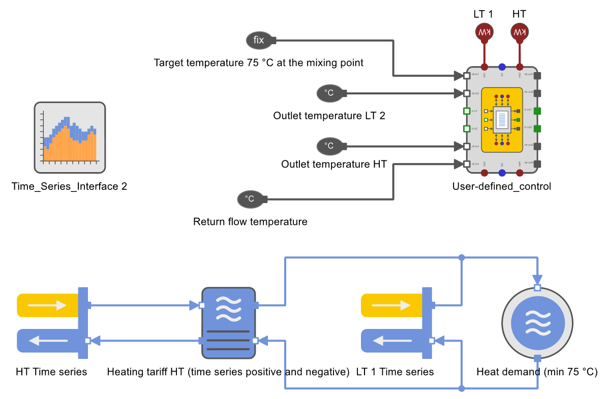
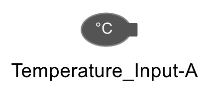
The two heat generators are assigned with time series for the varying outlet temperatures. These are read out via the components Temperature_Input-A (temperature sensor, see following figure).
In the User-Defined Control component, the factor \( c \), which describes the heat quantity ratio, is calculated.
You can also use the control elements for Addition, Subtraction, Multiplication, and Division +, –, *, and / from the component template folders Programmable Controls → Calculations to express the calculation operations. Because of the extensive arithmetic operations, this method is not very clear. Therefore, the User-Defined Control is preferred. In the Input Data of this component, the calculation steps can be viewed in the PML input window (PML-Eingabe), which is located under the heading Control.
The proportion \( \alpha \) of the respective mass in the total mass flow is defined. The mass balance at the mixing point is:
\( \begin{equation} \begin{aligned} \dot{m}_{mix} &= \dot{m}_{HT} + \dot{m}_{LT} && \qquad(2),\\[.3cm] \dot{m}_{HT} &= \alpha \cdot \dot{m}_{mix} && \qquad(3),\\[.3cm] \dot{m}_{LT} &= (1-\alpha) \cdot \dot{m}_{mix} && \qquad(4).\\[.3cm] \\ \end{aligned}\end{equation} \)The energy balance is:
\(\\ \begin{equation} \begin{aligned} \dot{H}_{mix} &= \dot{H}_{HT} + \dot{H}_{LT} && \qquad(5),\\[.3cm]\dot{m}_{mix} \cdot h_{mix} &= \dot{m}_{HT} \cdot h_{HT} + \dot{m}_{LT} \cdot h_{LT} && \qquad(6).\\[.3cm] \\ \end{aligned}\end{equation} \)If the mass flows are replaced by the definition from equations 3 and 4, the result is:
\(\\ \begin{equation} \begin{aligned} \dot{m}_{mix} \cdot h_{mix} &= \alpha \cdot \dot{m}_{mix} \cdot h_{HT} + (1-\alpha) \cdot \dot{m}_{mix}\cdot h_{LT} && \qquad(7),\\[.3cm] h_{mix} &= \alpha \cdot h_{HT} + (1-\alpha) \cdot h_{LT} && \qquad(8).\\[.3cm] \\ \end{aligned}\end{equation} \)The reduction by the heat capacity assumed to be constant and the conversion to \( \alpha \) are carried out:
\( \begin{equation} \begin{aligned} T_{mix} \cdot c_{p\ mix} &= \alpha \cdot T_{HT} \cdot c_{p\ HT}+ (1-\alpha) \cdot T_{LT} \cdot c_{p\ LT}&& \qquad(9),\\[.3cm] T_{mix} &= \alpha \cdot T_{HT} + (1-\alpha) \cdot T_{LT} && \qquad(10),\\[.3cm] T_{mix} &= \alpha \cdot (T_{HT} – T_{LT}) + T_{LT} && \qquad(11),\\[.3cm] \alpha &= \frac{T_{mix}-T_{LT}}{T_{HT}-T_{LT}} && \qquad(12).\\[.3cm] \\ \end{aligned}\end{equation} \)The generated heat quantities are calculated as follows:
\( \\ \begin{equation} \begin{aligned} \dot{Q}_{LT} &= \dot{m}_{LT} \cdot c_p \cdot (T_{LT} – T_{return}) && \qquad(13),\\[.3cm] \dot{Q}_{LT} &= (1-\alpha) \cdot \dot{m}_{mix} \cdot c_p \cdot (T_{LT} – T_{return}) && \qquad(14),\\[.3cm] \dot{Q}_{HT} &= \dot{m}_{HT} \cdot c_p \cdot (T_{HT} – T_{return}) && \qquad(15),\\[.3cm] \dot{Q}_{HT} &= \alpha \cdot \dot{m}_{mix}\cdot c_p \cdot (T_{HT} – T_{return}) && \qquad(16),\\[.3cm] \frac{\dot{Q}_{HT}}{\dot{Q}_{LT}} &= \frac{\alpha}{1-\alpha} \cdot \frac{T_{HT}-T_{return}}{T_{LT}-T_{return}}&& \qquad(17).\\[.3cm] \\ \end{aligned}\end{equation} \)Equations 12 and 17 are decisive because they form the calculation rule for the heat quantity ratio for observing the minimum mixing temperature (set temperature).
With the listed equations the constant factor \( c \) was calculated for the first example.
In the User-Defined Control, the equation 12 for the calculation of an auxiliary quantity \( \alpha \) introduced here is stored and the constant \( c \) is defined:
\( \begin{equation} \begin{aligned} \alpha &= \frac{T_{mix}-T_{LT}}{T_{HT}-T_{LT}} && \qquad(12),\\[.3cm]c &= \frac{\alpha}{1-\alpha} \cdot \frac{T_{HT}-T_{return}}{T_{LT}-T_{return}} && \qquad(18).\\[.3cm] \\ \end{aligned}\end{equation} \)
Because the mixing temperature should only be at least and not exactly reached, the following inequality was formulated in the User-Defined Control instead of equation 17 of the derivation:
\( \begin{equation} \begin{aligned} \frac{\dot{Q}_{HT}}{\dot{Q}_{LT}} &\ge \frac{\alpha}{1-\alpha} \cdot \frac{T_{HT}-T_{return}}{T_{LT}-T_{return}} && \qquad(19).\\[.3cm] \\ \end{aligned}\end{equation} \)According to equation 1 applies:
\( \begin{equation} \begin{aligned} \frac{\dot{Q}_{HT}}{\dot{Q}_{LT}} &\ge c && \qquad(20).\\[.3cm] \\ \end{aligned}\end{equation} \)This default can be changed individually.
High temperature > set temperature > low temperature.
Cases in which this condition is not met must be covered in the control with if-else constructions and their own calculation rules.
In the tutorial, the following three case distinctions are implemented as if-else constructions in the User-Defined Control.
Low Temperature Equal to High Temperature
If the low and high temperatures are the same, \( \alpha \) (in equation 12) would strive toward infinity. Because this is mathematically impossible, the bound is removed by setting \( \alpha = 0 \) for this case.
High Temperature Equal to Target Temperature
If the high temperature is equal to the target temperature, \( \alpha \) (in equation 12) would take the value 1, and \( c \) (in equation 18) would strive toward infinity. Because this is mathematically not possible, in this case \( \alpha = 0 \) is set. A second auxiliary size \( \beta \) is introduced, which in this case prohibits low temperature heat production:
\(\begin{equation} \begin{aligned} \\ Q_{LT} \le \beta \cdot 1000 && \qquad(21).\\[.3cm] \end{aligned}\end{equation} \)
The value 1000 is the so-called Big M and must be chosen greater than the maximum possible heat quantity.
High Temperature Lower Target Temperature
If the high temperature is lower than the set temperature the condition changes in the opposite direction. The system for calculating \( \alpha \) and \( c \) was therefore applied with swapped rolls for the low and high temperature. The resulting sizes were called \( \alpha_{2} \) and \( c_{2} \). These bounds are also implemented in the User-Defined Control component.
Structurally Different Energy Systems
The method shown is suitable for the application described above. Furthermore, the calculations can be extended. In the model of the following scheme (from the Simulation node HT, LT-1, and LT-2 heat generation with varying flow temperature in the tutorial) the bounds for three heat generators are calculated.

The calculation is done as above, but using the basic equations of thermodynamics. Boundary conditions for the MILP problem are formulated from the mixture equations. Two conditions can be derived for three generators:
\( \begin{equation} \begin{aligned} \dot{Q}_{HT\ sect.\ 1} &\ge c_1 \cdot \dot{Q}_{LT\ 1}&& \qquad(22),\\[.3cm] \dot{Q}_{HT\ sect.\ 2} &\ge c_2 \cdot \dot{Q}_{LT\ 2} && \qquad(23),\\[.3cm] \dot{Q}_{HT\ sect.\ 1} + \dot{Q}_{HT\ sect.\ 2} &= \dot{Q}_{HT} && \qquad(24).\\[.3cm] \\ \end{aligned}\end{equation} \)The constants \( c1 \) und \( c2 \) are calculated in the same way as above. The prerequisite is that the temperatures of both low-temperature suppliers are below those of the high-temperature suppliers. Otherwise, several case distinctions must be made as above. For other cases, such as varying outlet or target temperatures, these calculations must be made individually. This article cannot cover all existing cases. It shows only examplarily how such bounds can be calculated with the basic thermodynamic equations.