Peak Load Time Windows
Peak load time windows (high load time windows) are the times of expected highest network loads calculated annually by the network operators according to the uniform procedure of the Federal Network Agency and published in advance. With approved atypical network use on weekdays, i.e., the waiver of peak loads during high-load time windows, Energy demand costs, also named network charges, service price, performance price, power costs, grid usage charge, and demand rate) for large consumers can be reduced. These reduced grid usage fees provide the incentive for atypical grid usage. Atypical grid usage pursuant to Section 19 of the Electricity Grid Fees Ordinance (StromNEV) is intended to relieve the electricity grid at peak load times on the consumer side and lead to an optimization of grid utilization. A materiality threshold applies: the peak load in the peak load time window must be at least a certain percentage lower than the annual peak load. The following table shows an example of the peak load time windows for the Berlin power grid in 2023.
| Withdrawal Voltage | Winter 01/01 – 02/28; 12/01 – 12/31 | Spring 03/01 – 05/31 | Summer 06/01 – 08/31 | Fall 09/01 – 11/30 | Threshold of Significance |
|---|---|---|---|---|---|
| High voltage | 9:45 – 19:45 | - | - | 16:15 – 19:00 | 10 % |
| Medium voltage | 11:00 – 19:45 | - | - | 16:30 – 19:00 | 20 % |
| Low voltage | 16:30 – 19:45 | - | - | 17:15 – 19:15 | 30 % |
The maximum power that can be drawn within the peak load time windows is limited. For the calculation of the demand costs for the entire year, only the maximum demand within the peak load time windows is taken into account. Because this is lower than the maximum demand for the entire year, there is a financial advantage. For example, if the maximum power of 100 kW at a power cost of 60 EUR/kW per year is reduced to 70 % in the peak time windows, the individual power costs are calculated as follows.\begin{equation} \begin{aligned} 70 \ \text{kW} \cdot 60 \ \text{EUR/kW} &= 4.200 \ \text{EUR} \end{aligned} \end{equation}
A consumer in the medium-voltage grid with a maximum annual load of 10 MW and a maximum load in the peak load time windows of 7 MW pays a demand price of 80 EUR/kW. The general demand price is calculated as follows.
\begin{equation} \begin{aligned} 10.000 \ \text{kW} \cdot 80 \ \text{EUR/kW} &= 800.000 \ \text{EUR} \end{aligned} \end{equation}
The exceedance of the materiality threshold is verified in the following calculation.
\begin{equation} \begin{aligned} \dfrac{10 \ \text{MW} – 7 \ \text{MW}}{10 \ \text{MW}} &= 30 \ \% \\ \\ 30 \ \% &> 20 \ \% \end{aligned}\end{equation}
The individual demand price (performance price, grid usage price) is calculated as follows.
\begin{equation} \begin{aligned} 7.000 \ \text{kW} \cdot 80 \ \text{EUR/kW} &= 560.000 \ \text{EUR} \end{aligned} \end{equation}
Optimizing the Atypical Grid Usage in Peak Load Time Windows
TOP-Energy allows you to optimize atypical grid usage during peak load time windows. The following chart shows the difference in electricity and fuel costs at the peak time window peak loads of 73 MW, 69 MW, and 66 MW from the reference case. The optimal peak load during the peak load time windows is at the point where the sum of electricity and fuel costs is lowest.

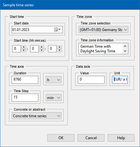
To take the peak load time windows into account, two time series must be stored in TOP-Energy: the time series with the demand prices corresponding to the peak load time windows in the tariff component and the time series with the reduced maximum power during the peak load time windows in the supplier component. To do this, carry out the following steps.
1. Create a time series for the demand costs in which the value is equal to the demand costs in the peak time windows and the value is equal to 0 outside of the peak time windows.