Serial Connection of Heat Generators With Different Temperature Levels
This article explains how to deal with the integration of low- and high-temperature heat generators into an energy system with a series connection using the tutorial 62 as an example.
The article is aimed at experienced TOP-Energy users, since the complex issues require a profound understanding of the simulation and optimization processes.
The problem described occurs when the heat demand in a project is to be covered by (at least) two generators with different outlet temperatures and the lower temperature level is too low for the demand.
Problem Description Using an Example
In the present energy system, a heating requirement at a temperature level of 60 °C is to be covered by a combination of two generators. A geothermal plant supplies energy at a temperature level of only about 35 °C. Therefore, a power-to-heat system must be used for heating. For the following consideration it is assumed that the power-to-heat system is “more expensive”, i.e., here: it consumes more electricity per generated kilowatt hour of heat.

If an operational optimization is carried out with the model shown in the illustration above, the computationally correct, but technically impossible behavior results, with which the geothermal plant is operated because of the smaller costs with maximum output and the technically conditioned maximum temperature of the geothermal plant of 35 °C is exceeded. The power-to-heat system is therefore only switched on if the output of the geothermal system is insufficient.
In the following, possibilities are shown to map the desired, technically realistic, behavior in TOP-Energy without specifying the outlet temperature of the geothermal system. There are three different cases:
Case 1
If the rated output of the geothermal system is much lower than the heat demand, the systems can be connected in series without further intervention. The prerequisite for this is compliance with the conditions for series connection.

The Outlet temperature of the geothermal system may not be preset, but must be set to Calculated value by right-clicking. After the simulation, a check of the calculated Outlet temperature, which is displayed under Input data → Technical input data, can ensure that the conditions have been met and plausible results have been generated.

Because then the inlet and outlet temperatures of the low-temperature heat generator would be fixed (the inlet would be determined by the outlet at the heating demand), the mass flow would be clearly determined by the following equation.
\(\dot{Q}\) is also defined as a result of the optimization problem.
The same applies to the next component connected in series, the high-temperature heat generator: The mass flow is determined by the temperature ratio. Since the same mass flow must flow through both heat generators due to the series connection, this equality cannot be achieved in most cases.
Case 2
In this case there is a very large heat reservoir at a low temperature level, whose heat can be provided cheaply. The problem that the outlet temperature of the low-temperature generator circuit is not high enough for the demand can be countered by clever manipulation of the optimization. Although temperatures cannot be directly anchored in the heat cycle to limit the optimization problem, the optimization can be influenced in such a way that the temperature limits are maintained.
The basic idea is to couple the output of the two generators so that the cheaper low-temperature generator cannot supply all the energy but is set in relation to the high-temperature generator and thus limited. This ratio can be calculated by the ratio of temperatures:
The equations for the heat generation of the high-temperature (HT) and low-temperature (LT) generators are as follows:
\(\dot{Q}_{HT} =\dot{m} \cdot c_p \cdot \Delta T_{HT} \\\dot{Q}_{LT} = \dot{m} \cdot c_p \cdot \Delta T_{LT}\\\)
In the present example:
\(\dot{Q}_{HT}= \dot{m} \cdot c_p \cdot (60°\!C – 32°\!C) \\\dot{Q}_{LT} = \dot{m} \cdot c_p \cdot (32°\!C – 24°\!C)\\ \)
The quotient low temperature to high temperature is calculated as:
\( \begin{equation} \begin{aligned} \dfrac{\dot{Q}_{LT}}{\dot{Q}_{HT}} &= \dfrac{\dot{m} \cdot c_p\cdot (32°\!C – 24°\!C)}{\dot{m} \cdot c_p \cdot (60°\!C – 32°\!C)} \\&= \dfrac{32°\!C – 24°\!C}{60°\!C – 32°\!C} \\ &= 0,3 \end{aligned}\end{equation}\\\)
In the example of Tutorial 62 in Variant 2, the heat pump represents a favorable source from a large energy reservoir. According to the above calculation, however, this may only provide about one third of the total heating energy required.

The TOP-Energy solution is implemented by using the components of the programmable control.
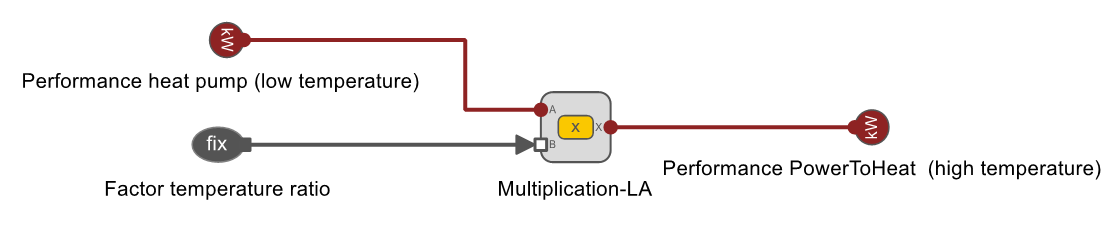
The following equation is represented by the interconnection of the corresponding logic elements and must be observed in each simulation step:
\(\dot{Q }_{LT} \cdot \dfrac{60°\!C – 32°\!C}{32°\!C – 24°\!C} = \dot{Q}_{HT} \\\)As a result of the simulation, the outlet temperature of the heat pump is 32 °C at any time (note that it is a calculated value and this was not specified).

If the heat demand is so high and the nominal power of a heat generator is so low that even at full load of the low heat generator the heat demand cannot be covered while maintaining the prescribed ratio of the heat generators, there is no solution. If one of the heat generator components reaches its maximum load, the other cannot produce more because of the fixed ratio. If, for example, the systems Power-to-Heat with a Nominal Thermal Power of 100 kW and heat pump with a Nominal Thermal Capacity of 10 kW are to be operated only in combined operation in a fixed ratio of 2:1, a heat requirement of 60 kW is inevitably divided into 40 kW (power-to-heat) and 20 kW (heat pump). Due to the fixed ratio, the two systems only achieve a total nominal power of \( 2 \cdot 10\, kW_{P2H} + 1 \cdot 10\,kW_{heat~pump}\). The performance of the power-to-heat system cannot therefore be fully exploited by this modeled restriction.
Case 3
If the requirements for the energy system cannot be fulfilled by case 1 or 2, there is a third possibility to influence the optimization problem.
In variant 3 of the tutorial, a connected cooling circuit serves as a low-temperature source. The waste heat from the vapor-compression refrigeration system (VCRS) can be fed out and integrated into the heat cycle. However, the cooling demand fluctuates so strongly that the waste heat is available in excess at certain times and insufficiently at others.

The implementation in TOP-Energy is similar to case 2. The temperature ratio of the heat generators is calculated to implicitly limit the outlet temperature of the low-temperature heat exchanger (Heat_Release_To_Warm_Water from the Heat transfer Component template library folder). In contrast to case 2, the logic components are extended so that the ratio does not have to be rigidly maintained, but only represents a barrier for the maximum generation of low-temperature heat.

Detailed descriptions of the components of the programmable control can be found here.
This is the equation mapping the logic elements figured:
\( \dot{Q}_{HT} \cdot \dfrac{32°\!C – 24°\!C} { 60°\!C – 32°\!C }>= \dot{Q}_{LT}\\\)The result in TOP-Energy shows the desired behavior: The capacity of the heat exchanger (LT) (Heat_Release_To_Warm_Water) is implicitly limited so that the maximum amount of energy that can be supplied is such that a temperature increase in the Heat_Release_To_Warm_Water component to 32 °C takes place. In cases where excess low-temperature heat is available from the cooling circuit, it must be dissipated through the recooler. This behavior can be seen in the following diagram: If the outlet temperature of the heat exchanger (in °C, red line) is less than 32 °C, the heat exchanger does not have to provide any cooling capacity. As soon as the 32 °C is reached, an additional cooling capacity (in kW, blue bars) must be provided by the heat exchanger.

Summary
The proposed solutions presented here are intended to clarify the concept of logic components for influencing the optimization problem. Depending on the application, the solution can be adapted or extended (e.g., temperature curves for outlet temperatures can be entered into the logic formulation).
The concept of temperature level dependent power coupling of the units can also be applied for parallel connections. The article Heat generators with different temperature levels (parallel connection) describes the special features to be considered for parallel connections. It is up to the user to decide which technical system can be best represented in which way.